Isokinetics machines are measurement devices. They provide us with information about the moving mechanical performance of muscle groups. They assume (very incorrectly) that the muscles they are testing move at a constant angular velocity (or in other words that the muscle move isokinetically). Unfortunately, most biological joints do not possess a fixed axis of rotation and hence the machine will make errors. The extent of the error will depend on the joint tested and the position of the subject.It is possible to measure multi joint motion and moment using the machine. It is generally understood that isokinetic refers exclusively to the motion of the mechanical elements external to the body (not the body itself).
Each of the systems available has its own features but basically they are all the same in that they have a rotating center shaft which moves via attachments in either a single plane or multiple planes (take note – this allows for the reproduction of many movements e.g. diagonal movements at the shoulder are reproducible through single plane motion at a specific angle, whilst multi plane motion e.g. throwing a ball, is available through a cord wrapped around a coil attached to the shaft).
Remember you set the velocity of the turning shaft by entering the isokinetic speed which the machine will try to stay at throughout most of the motion.
There are many parameters which must be set in advance to control the test/exercise. These vary somewhat between individual joints, however, there are some general rules.
The machine needs to be told the range of motion through which to move known as the ROM. This is measured in degrees and describes the total allowable angular displacement of the attachment. It should not be confused with the motion taking place at the joint (which is often even further removed by the misalignment of the instantaneous axis of rotation). It is normal to describe this motion in relation to the joint/s being tested and will always be referred to in one contraction cycle. For example if you are testing the elbow you might go from straight (0 degrees) to bent at 90 degrees. This would give a ROM of 0-90 degrees or 90 degrees in total. In reality each repetition would be straight (0 degrees) to 90 and then back to straight. But an isokinetics machine only needs to know where it is going from and to: So the range is 0-90.
Angles of peak torque:At each joint, for each major muscle group, there is a point within the range where the muscular advantage, and lever disadvantage, give the correct balance to allow peak force / torque to be produced. The torque produced at this point will be the highest that can be produced in that movement. This is referred to as the angle of peak torque. When setting the range of motion it is always best practice to try to encompass the angle of peak torque for each of the muscle group/s tested. In concentric / concentric contractions this will normally be the angles of peak torque for two different muscle groups which can complicate the situation. The total range of motion must also account for any acceleration and deceleration phase (see below) to ensure the angle of peak torque is included in the isokinetic part of the range of motion.
Magnitude of ROM: There is evidence to suggest that an increase in peak moment will be experienced with increasing ROM i.e. if you test the knee over a 90 degree ROM and then over a 120 degree ROM you should expect an increase of approx. 9% in peak moment. This may be due to tension developments or greater neural activation within a muscle.
The total range of motion in each contraction cycle can be separated into three parts:
- Acceleration.
- Isokinetic ROM (IROM).
- Deceleration.
The isokinetic range of motion is always smaller than the total range of motion as each contraction cycle starts and terminates at a static position i.e. if we set a test speed of 60 degrees/second at the beginning of each movement the machine has to allow acceleration to 60 then at the end of each movement the segment has to be decelerated back to 0 degrees per/second. This takes time and reduces the total isokinetic range (see here for full description).
Angular Velocity: This is usually measured in degrees/second but you will often see it stated as radian/second (one rad is approx. 57.3 degrees). Remember that pre-set velocity cannot be related to muscle linear contraction velocity (as described by Hinson et al 1979). It should be noted that the higher the angular velocity the less movement will be performed isokinetically as the acceleration phase will generally take longer this can be measured and used as a descriptor of explosive power / strength.
Pre Set Speed: All systems when used isokinetically work on the same principle. The input attachment (the bit you attach the patient on to) moves at a pre-set angular velocity (PAV).
Now the user can push or pull or twist etc. etc. as hard or as little as they like and the machine will only move at the speed at which you have set. In reality the machine moves to the speed and actually within small boundaries around that speed known as the pre set angular velocity margins or PAV margins. This variance is within small boundaries of the speed you set. If the user pushes harder the speed does not increase but the resistance does and the movement is maintained within these very narrow margins about the PAV. But it takes the machine an amount of time to adjust to increases and decreases in force.
Say the subject hits the speed set for isokinetic motion but then produces even more force, the machine will see a change in the force and adjust accordingly, however, during the adjustment the speed may increase slightly above the pre set speed. Conversely if the resistance drops the speed may also drop until the machine adjusts and reduces the pressure allowing the speed to recover.
SAMPLE RATE: This adjustment occurs at different rates in different machines and is known as the sample rate (or the amount of times per second the machine can adjust). The higher the sample rate the smoother the motion. Old machines sample at 100hz or 100 times per second. this is fine in slower motions around large turning circles as it gives the machine plenty of time to adjust, however at higher speeds around smaller motions the machines can have very little time to adjust making the movement jerky and often not even isokinetic. New machines can sample at up to 5khz (5000 samples per second – CSMI Norm samples at 5khz) they are able to produce smooth movement even at high speed around small ranges of motion and this has been the biggest advance with modern computing technology.
If the user pushes with a force unable generate the speed required for the lower margin of the PAV then the system will interpret this as the user wishes to stop (this will often be seen as a jerky movement on the machine).
The width of the PAV margins are a performance characteristic of each individual system which are often unchangeable (Kin-Com, Isocom, Isomed, Biodex, Con-Trex) but can be altered on some systems (Cybex Norm (sensitivity)).
Remember, the moment (force) generated does not have to be maximal but it has to be enough to generate the PAV otherwise the machine will not run (or in other words, if the machine stutters and jerks then the speed needs to be turned down (or the PAV altered if available) as the movement is actually isotonic whilst this happens (click here for a full description of PAV).
Damp Settings:At the end of the acceleration phase before the movement reaches isokinetic values there will often be a spike at the beginning of the contraction. This has been referred to as the ‘Impact Artefact’ (or torque overshoot, impact torque, moment overshoot or overshoot). This spike does not represent muscle performance at the pre-set velocity they are actually simple bio-mechanical interaction between the subject and the machine. They occur in the acceleration and deceleration phases (often called moment signal transience). These sectors are usually equal to the ROM and speed respectively (e.g. over 90 degrees at 30 degrees/second the transient phase will be equal to 1 degree at either end of the ROM). As they are not representative of force developed by the musculo skeletal structures they are most often removed or damped. Dampening the signal reduces the spikes in the reults (see below).
More modern dynamometers allow for this problem by using ramping or computer controlled acceleration. This is one reason why strength results cannot be compared from one make to another.
Although the overshoot is not meaningful with regards to peak moment it is very important as a reflection of the capacity to recruit the neuromuscular apparatus and generate a moment. For this reason most good dynomometers will allow you to alter the damp settings on a manual basis so both aspects can be investigated.
For an in depth review of moment artifact please click here.
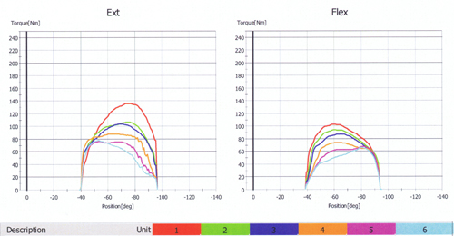
Moment angle position curves: MAP curves are generated after each isokinetic repetition. In essence they are the recorded values at each point in range of motion (for which there is a measurement). They are referred to as curves but will often be flat or odd shapes (differing shapes are known as perturbations and are often analysed to give meaningful data as to the Musculo-skeletal performance). Normal MAP curves always start from 0 (both velocity and force) then raise to the point of mechanical and muscular efficiency. From there they fall back (partly due to the deceleration of the machine) to 0 once again. The most common shape of MAP curve is the inverted U seen below.
Isometric Pre-activation: This refers to the machine waiting (isometrically) until a certain amount of force has been developed by the muscles before motion is allowed to occur. This static tension generated in the muscles is often called pre-loading. This was first described by Gransberg and Knutsson (1983) who said it had a restraining effect on the initial moment oscillations.
In recent years allot has been made of this effect either before or even during concentric or eccentric contractions. Biodex have called this effect impact free acceleration in the concentric mode and reactive eccentric mode. Con Trex have used the principle to offer ballistic mode to limit inertia (along with predicting strength and speed). Cybex and CSMI have always allowed the amount of pre-activation to be selected manually and have also allowed a different level to be chosen during the contraction phase up to the upper limit of the dynomometer. The Cybex and CSMI method offers the best overall control but requires more skill to use.
Lower Isometric Bias:This term is used interchangeably with isometric pre activation and is also called minimal start and back forces. It describes the amount of moment that has to be maintained in order to ensure smooth progression of isokinetic motion and it can be used to replace or compliment isometric pre-activation.
Upper Moment Limit. This is the maximal moment that may be exerted by the machine against the subject. It was incorporated to ensure the safety of vulnerable structures e.g. ACL after reconstruction, but it may also be used for the purpose of fine motor performance analysis. In recent years this concept has been used to allow the new machines to offer forced continuous passive motion (FCPM). Now the machine is given an upper limit to push to and is allowed to pressthe motion to force extra movement at a particular joint. When used with range of motion expansion this method has proved highly successful in rehabilitation particularly in patients who have had joint replacement.
Feedback.Can be either auditory or visual (the visual feedback varies wildly between machines). Both can have profound effects on performance (up to 30% Dvir 1995). In a testing situation (where feedback is not a variable) the feedback to the subject should be kept to a minimum. In the training / exercising situation the feedback should be set to allow maximal performance from the subject.
Length-Tension Relationships. The most basic relationship governing muscle performance is often said to be the association between the length of the muscle and the corresponding tension it produces. The easiest way to understand this is to think of an isometric contraction. If we started with a muscle in a loose position the tension of that muscle could be recorded using a dynamometer. As the muscle is slowly lengthened a point would be reached where passive resistance is recorded. The muscle would continue to be lengthened until no increase in tension was apparent. Two independent sources of resistance could then be identified.
- The active tension produced by the contractile elements.
- The passive tension produced by the non-contractile elements.
The muscle tension corresponding to the maximal active tension is known as the resting length (physiotherapists often confuse this length with the anatomical position). Gordon et al. (1996) stated that the length-tension relationship of the whole muscle reflects the mechanical behavior of the individual fibers which can be related to the number of cross bridges between the actin and myosin filaments in the fibers (or the degree of overlap).
Real World Strength. No matter what techniques we use (either isometric, isokinetic or other) to measure strength (not to be confused with force as this is a linear entity) we actually look at the rotational effect generated by the force of a muscle or muscle group. So, in other words, we actually infer the force generated by the muscles rather than record it.
Gravitational Correction. Since the majority of isokinetic tests consist of angular motions e.g. plantar and dorsiflexion of the ankle, the effects of gravity must be corrected for. However, in some movements e.g. inversion and eversion of the ankle, gravity does not have to be corrected for even though the motion is angular.
This is extremely important when considering the agonist/antagonist strength ratio. Consider it like this. The weight of the lower leg has to be overcome by the quadriceps to extend the knee in the sitting position, yet when the knee is flexed by the hamstrings the weight of the leg actually assists the movement. So gravity correction becomes important for reliable results.
Force-Velocity Relationship. There is a direct relationship between the amount of force generated and velocity in that:-
- For concentric contractions there is a parallel decrease in the maximal moment developed by the muscles as speed increases. This is because of neuromuscular recruitment patterns i.e. both type I and II fibers are activated together at lower speeds but as speed increases less type I fibers are recruited and eventually become inactive. At very high velocities smaller and smaller fiber populations are recruited (Kannus 1994).
- For eccentric contractions the maximal moment may rise initially but at higher velocities it plateaus due mainly to neuromuscular facilitation (as eccentric contractions could be theoretically very high at speed Perrin 1993).
Order of Strength. The principles mentioned above are supplemented by:-
- At the same velocity eccentric strength is greater than concentric strength at medium joint speeds.
- Elftman’s (1966) principle states that the order of strength is dependent on contraction mode i.e. eccentric is greater than isometric which is greater than concentric.
- These are also dependent on the type of exercise performed i.e. isokinetic is greater than isometric which is greater than isotonic
A further expansion of these principles can be seen here.
Order of Joint Forces. When a muscle is contracted around a joint a certain amount of pressure is created within that joint.
- That pressure is dependent on the type of exercise i.e. isotonic is greater than isokinetic which is greater than isometric
- And also the type of exercise i.e. eccentric is gretaer than isometric which is greaer than concentric.
A further expansion of these principles can be seen here.
Test Velocities. For concentric contractions most dynamometers have a maximum speed of 500 degrees per second. The use of velocities is dependent on the joint tested and the ROM, however, higher velocities are usually only of academic interest. Corresponding eccentric velocities are not usually possible and are generally one-third less than concentric. Stretching an active muscle at high velocity poses a serious threat to muscle integrity (so don’t do it). Restraint of antagonist activation (or in other words when the antagonist muscles activate to prevent hyper extension) is a neuromuscular phenomenon that is well developed in athletes (Glossman et al. 1988). This is not so well developed in untrained athletes who may find high velocities very difficult.
Increased Eccentric Contraction. Theoretically the eccentric strength could exceed the isometric strength (never mind the concentric strength) by about 100% (Edman et al. 1979). However, in real life this never happens. The best explanation for this phenomenon suggests a negative feedback loop which involves peripheral and spinal regulation in order to avoid excessive stresses on the muscle (Storber, 1989). The only time this feedback loop can be over-ridden is when the CNS determines that increased eccentric contraction is needed for defensive purposes. When this happens there is usually damage to the musculo-tendinous junction rather than the muscle.
The Eccentric/Concentric (EC) Ratio. This is expressed as the maximal eccentric moment divided by the maximal concentric moment. Since this is dependent on velocity it should increase proportionally with this. It has been proposed that with respect to single joint testing (Dvir, 1994) the EC value derived from low to medium test velocities is very likely to be within the range of 0.95 : 2.05. Trudelle-Jackson et al. (1989) proposed that the EC ratio at slower speeds is less than 0.85. This ratio tends to fall particularly in the presence of pathology (Conway et al. 1992). Bennett and Storber (1986) have suggested that a particularly low EC ratio (less than 0.85) is a potential source of patella-femoral pain (based on an error in neuromotor control). If there is a large increase in the EC ratio then excessive connective tissue components may be the reason. As described by Dvir and Dagan (1994) this may be due to a rare form of hereditary anemia which should be eliminated before continuing with isokinetics.
Closed versus Open Chains. Most isokinetic machines are configured for assessing planar, single joint motion. However, in most instances joint motion is multi planar and often combined harmoniously with other joints. Although moment output may not be measurable from the individual contributions of the muscles responsible for executing multi joint motion, their use is of considerable interest. A lot of debate rages over the use of closed chain and open chain exercises. It is true that there are high joint loading forces during most isokinetic movements. Obviously if a load is to be moved it must be supported by structures around the joint. As most muscles have very short levers only a small percentage of the muscle force is used to counteract the external load. The rest is transmitted through the joint articular surface or taken up by anatomical structures such as the ligaments and capsule. It should be emphasized that the forces seen during isokinetics are not the largest the joint will be expected to support.
The following are several examples of forces:-
- Kaufman et al (1991) indicated average tibio-femoral force of 4 times body weight whilst testing isokinetically. This is equal to that obtained during walking.
- The anterior shear force was on average 0.3 times body weight which is higher than that expected during walking but lower than that expected during stair climbing (1.7 x body weight) or running (3 x body weight).
- Posterior shear force was on average 1.7 times body weight which is larger than walking but on a par with stair climbing and lower than running.
- Patella-femoral forces reaching 5.1 times body weight at 60 degrees/second were calculated. This can be compared to 0.5 times body weight during walking, 3.3 times body weight whilst ascending stairs, 7.6 times body weight in the squat or 20 times body weight during jumping.
Eccentric-Concentric Coupling. This phenomenon of concentric contraction potentiation following eccentric contraction is well established (Cavanagh et al 1968, Komi and Bosco, 1978/1979, Bosco et al., 1987). This phenomenon is also termed as pre-stretching, stretch shortening cycle or plyometric contraction. It is based primarily on the mechanical behaviour of the series elastic element found in contractile elements and tendons within the muscle (Svantesson et al. 1991). Basically in eccentric contractions energy is accumulated in both mechanical and chemical forms and is released at the beginning of the next concentric contraction. This is relevant to isokinetic testing as the plyometric response can be trained for. Affecting an increase in plyometric contraction using isokinetics is more controversial.